The Mandelbrot set
The Mandelbrot set became a familiar and popular shape after its discovery by Benoit Mandelbrot in 1980. It was not possible to predict that such a shape existed before we had computers able to display or print graphics. It arises from an extremely simple formula but only after many iterations. The formula is
zi+1 = zi2 + c
where z and c are complex numbers. The starting value of z is z0 = 0 + 0i. When the formula is applied repeatedly the value of z either stays within a small distance of the start or escapes towards infinity, this behaviour depending on the value of c. The boundary between these behaviours, plotted in the c-plane*, is the Mandelbrot set. It is an extremely complicated shape that has been proven mathematically to be a connected curve. It is usual to plot the exterior of this boundary with brightness (grey levels) proportional to the number of iterations it takes before z gets more than a certain large distance from the origin. Inside the boundary is just black (0).
* By c-plane I mean an Argand diagram for the values of c: the real parts form the horizontal axis and the imaginary parts are vertical.
Julia sets
Way back in the early 1900s a French mathematician called Gaston Julia had already investigated some properties of the formula. He could not have envisaged the intricate patterns involved in the sets of points now named after him. Again, these can only be made visible with computers.
This time, for a given value of c indicated by a click on the Mandelbrot set, we plot what happens to various starting values of z (the plot is in the z-plane).
Observe that for points outside the Mandelbrot boundary the corresponding Julia set breaks up into "dust" and for points inside the boundary there are significant black patches.
Precision
This program only uses the standard JavaScript Number precision with 52-bit mantissas. So zooming in many times will lose accuracy.
Extending the polynomial
This program enables adding further terms to the iterated formula, with coefficients that you can choose. The formula becomes
zi+1 = f1.zi + f2.zi2 + f3.zi3 + c
It is something to experiment with, or set both f1 and f3 to zero for the standard shapes. The coefficients are applied to both the Mandelbrot and Julia sets.
As well as setting the coefficients there are buttons [...] for animating any one of them through a sequence of values. Note that this only makes sense if at least two of the coefficients are non-zero.
I thank u/AbideByReason on Reddit for pointing out that the cubic term adds interesting effects. The post in r/fractals had f3 = 0.16 but it is worth exploring and even to use negative values.
Colour tables
There are a few colour tables to choose from. In their names you can see the order of red, green and blue going from darkest at the left to brightest. The slash characters indicate slopes of pure grey, going upwards or downwards.
For each pixel calculated for Mandelbrot or Julia we get a grey level in the range 0..255 which is used as an index in the selected colour table to look up RGB values for plotting. The tables are called LUTs (Look-Up Tables).
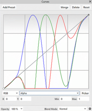
For example, the one called /BGR/ is like this (as first created in Affinity Photo):
Gamma
Gamma curves are useful for spreading the contrast range. This is explained on Wikipedia. I implement it as another look-up table indexed by the grey level result of the Mandelbrot/Julia calculator, before applying the colour table.
Arrow keys
By themselves the arrow keys move in the c-plane. Either the real or imaginary part, as appropriate for the direction of the arrow, is incremented or decremented by 0.1 divided by the zoom factor (the power of 2, not the index zoom level).
However, if the Ctrl key is also pressed (Apple: Cmd key, but I am unable to test this) the offsets are in the z-plane. In the case of Julia sets this just enables the image to be repositioned. The Mandelbrot set behaves differently: if the Ctrl-arrows are used a new line appears below the zoom level at the top of the control window, showing a value for z0. The Mandelbrot set is then distorted because z0 is a new starting point for the iteration, instead of 0 + 0i. This distortion can be interesting though.
How I created the colour tables
- In my GRIP program I created an 8-bit monochrome image 256 pixels square containing a gradient rising from 0 to 255 in unit steps from left to right.
- I saved that as a TIFF file (no compression to change anything) and opened it in Affinity Photo, where I applied the curves adjustment that I had made previously (as in the illustration above).
- Saving as TIFF and reopening in GRIP again I then measured a linear profile going horizontally across the whole image. GRIP has an option to save the profile in CSV format (comma-separated values as plain text).
- I opened the CSV file in Open Office Calc (the free equivalent of Excel) to delete unwanted columns from the table. Saved again as CSV this gave me comma-separated red, green, blue values that I could easily wrap as an array in Javascript.