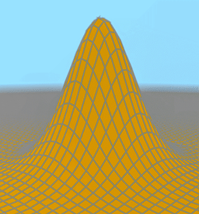
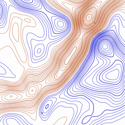
The 2-tone contour map uses brown to indicate hills raised above 0 (sea level) and blue for depths below 0. The program starts with a plain sheet at height 0. Two opposing particles then begin moving apart. There is a Gaussian hump (shown here). One of the particles adds this hump at its current position (shown by a brown cross) and the other particle subtracts exactly the same hump (at the position shown by a blue cross).
Gradually the shape of the hump changes. Its height and its half-height radius change by small random amounts. The velocity components of the two particles also change by small random amounts on each time-step.
On each step the two particles still use the one hump. So one particle is adding a certain volume and the other is subtracting the same volume. The total volume (under hills - above lakes) therefore remains zero at all times (in reality this is only approximate because the program does nothing special at the edges of the canvas).
When the height of the highest hill and the depth of the deepest lake differ by a certain threshold amount there is a phase of erosion until the maximum and minimum differ by less than another value. Then the particles resume their process. This ensures that the contours do not become too extreme and crowded.
I like to think there is an analogy with particle-antiparticle pairs springing from the vacuum, the total energy of the field remaining zero: complexity from nothing! But I am also fascinated by the resulting maps and the shapes implied.
The program is written in plain vanilla JavaScript in a simple HTML page. It uses a 2D canvas. The bulk of the processing time on each step is taken by drawing the contour map. I do not think that would be any faster using a WebGL canvas.
There is another program using the same script files in which you can experiment with placing the Gaussian humps yourself. As well as a map view you can see a perspective scene (as in the hump image above). This was intended to help people understand contour maps. That other program is here.
24.1.17 - Variant called Waterways shows both sets of contours brown, as if raised, and the areas
between them blue, like rivers.
Two versions now:
Waterways or
Auto-contours
21.1.1 - Fourth option added to map style drop-down: Coloured image
20.11.15 - This new version is faster when drawing contours only. On each time-step it redraws only the parts of the map that have been modified, rather than drawing the whole map each time. Speed is inversely proportional to the square of the half-height radius of the gaussian hump, which slowly varies by a random amount so it will sometimes speed up and slow down. Image display still requires the whole canvas to be redrawn because of using the full height range for brightness scaling.
20.10.28 - First version made public.